Design of a Single-Zone CAV System#

In this notebook a single-zone, constant air volume (CAV) air conditioning system is designed with the package hvac.air_conditioning. The examples are taken from the book Heating and Cooling of Buildings by T. Agami Reddy, Jan F. Kreider, Peter S. Curtiss and Ari Rabl (3th Edition, 2017), Chapter 19.

from hvac import Quantity
from hvac.fluids import HumidAir, Fluid
from hvac.air_conditioning import AirConditioningProcess, AdiabaticMixing, AirStream, SpaceConditionLine, Fan
from hvac.charts import PsychrometricChart, StatePoint

Q_ = Quantity

The general layout of an air conditioning system is shown in the figure below.

scheme

A. Summer Peak Design#

A space is to be maintained at 78°F (25.5°C) dry-bulb temperature and 50% RH. The total cooling load (heat to be removed from the space to maintain comfort) is 120.000 Btu/hr (35 kW) of which 70% is sensible heat. Ventilation air at 1000 ft³/min (472 L/s) is required on the peak day when the outdoor conditions are 95°F (35°C) and 55% RH. The room supply air temperature is 20°F (11.1°C) below that of the room set point temperature (a typical value for commercial buildings at peak operating conditions). What are the space air supply ﬂow rate and the cooling coil rating (total cooling capacity and SHR)?

0. Design Conditions#

Zone air condition:

zone_air = HumidAir(Tdb=Q_(78, 'degF'), RH=Q_(50, 'pct'))

Cooling load on summer peak design day:

Q_zone = Q_(120_000, 'Btu / hr')
SHR_zone = Q_(70, 'pct')

Outdoor air condition:

outdoor_air = HumidAir(Tdb=Q_(95, 'degF'), RH=Q_(55, 'pct'))

Ventilation air flow rate:

V_vent = Q_(1000, 'ft ** 3 / min')

1. Determine the Supply Air Condition and Mass Flow Rate#

The design procedure starts with a reasonble choice of the supply air db-temperature:

T_supply = Q_(58, 'degF')

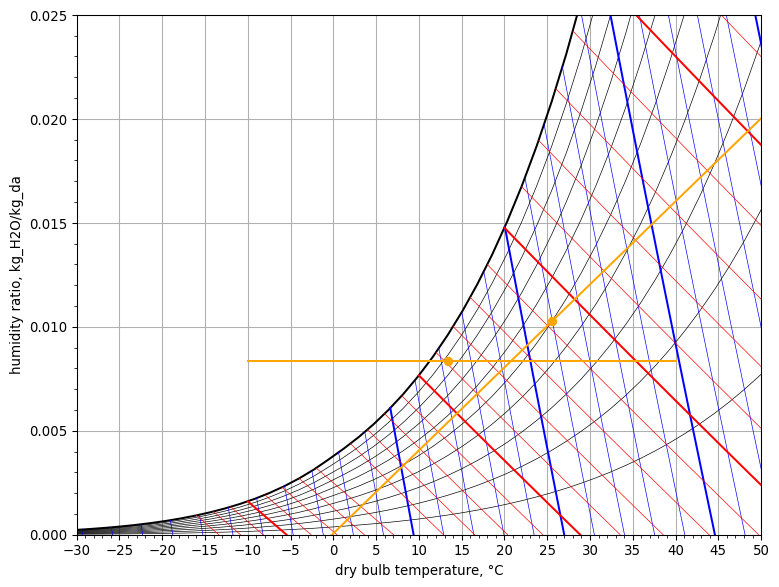
The possible states of the supply air in order to meet the zone load, must lie on the space condition line. The space condition line is determined by the zone air condition and the SHR of the zone.

space_condition_line = SpaceConditionLine(
    space_air=zone_air,
    Q=Q_zone,
    SHR=SHR_zone
)

psych_chart = PsychrometricChart(fig_size=(8, 6))
psych_chart.plot_space_condition_line(
    start_point=space_condition_line.start_point(),
    end_point=space_condition_line.end_point(),
    space_point=space_condition_line.space_point()
)
psych_chart.plot_line(
    name='line1',
    start_point=StatePoint(T_supply.to('degC'), Q_(0, 'g / kg')),
    end_point=StatePoint(T_supply.to('degC'), Q_(15, 'g / kg'))
)

psych_chart.show()

By choosing the supply air db-temperature, the supply air state is thus fully determined by the space condition line. Also, by specifying the supply air temperature, the required mass flow rate of supply air will be determined at the same time.

zone = AirConditioningProcess(
    T_ai=T_supply,
    air_out=zone_air,
    Q=Q_zone,
    SHR=SHR_zone
)
supply_air = zone.air_in
m_supply = zone.m_da

ja.display_list([
    f"supply air state: <b>{supply_air.Tdb.to('degF'):~P.1f} TDB, {supply_air.W.to('lb / lb'):~P.5f} lb<sub>w</sub>/lb<sub>da</sub></b>",
    f"supply air mass flow rate: <b>{m_supply.to('lb / hr'):~P.0f}</b>"
])

supply air state: 58.0 °F TDB, 0.00836 lb_w/lb_da
supply air mass flow rate: 17240 lb/h

2. Determine the Mixed Air Condition at the Entrance of the Cooling Coil#

First we determine the mass flow rate of outdoor ventilation air. As the supply air mass flow rate, which is the same as the mass flow rate of air through the cooling coil, has already been determined, the mass flow rate of recirculation air can also be determined.
When the states of outdoor ventilation and recirculation air, together with their mass flow rates, and the mass flow rate of air through the cooling coil are known, the air state at the entrance of the cooling coil can be determined from adiabatic mixing.

m_vent = outdoor_air.rho * V_vent
m_recir = m_supply - m_vent

ja.display_list([
    f"ventilation air mass flow rate: <b>{m_vent.to('lb / hr'):~P.0f}</b>",
    f"recirculation air mass flow rate: <b>{m_recir.to('lb / hr'):~P.0f}</b>"
])

ventilation air mass flow rate: 4160 lb/h
recirculation air mass flow rate: 13079 lb/h

outdoor_air_str = AirStream(state=outdoor_air, m_da=m_vent)
recir_air_str = AirStream(state=zone_air, m_da=m_recir)
mixed_air_str = AirStream(m_da=m_supply)

mixing_chamber = AdiabaticMixing(
    in1=outdoor_air_str,
    in2=recir_air_str,
    out=mixed_air_str
)
mixed_air = mixing_chamber.stream_out.state

ja.display_list([
    f"mixed air state: <b>{mixed_air.Tdb.to('degF'):~P.1f} TDB, {mixed_air.W.to('lb / lb'):~P.5f} lb<sub>w</sub>/lb<sub>da</sub></b>"
])

mixed air state: 82.1 °F TDB, 0.01254 lb_w/lb_da

3. Determine Fan Heat and Air State at Cooling Coil Exit#

The supply fan adds heat to the cooled air stream leaving the cooling coil due to inefficiencies of the fan and also of its motor, as it is also located within the airstream. To deliver the required mass flow rate of supply air to the space, the fan pressure rise in the example is 3 inWG. The efficiency of the fan is 70 %, while the fan motor efficiency is 84 %. The fan delivers the air to the space at the already determined supply air conditions.

supply_fan = Fan(
    air_out=supply_air,
    fan_pressure=Q_(3, 'inch_H2O_60F'),
    fan_efficiency=Q_(70, 'pct'),
    motor_efficiency=Q_(84, 'pct')
)
cooled_air = supply_fan.air_in

ja.display_list([
    f"cooled air state: <b>{cooled_air.Tdb.to('degF'):~P.1f} TDB, {cooled_air.W.to('lb / lb'):~P.5f} lb<sub>w</sub>/lb<sub>da</sub></b>"
])

cooled air state: 56.2 °F TDB, 0.00836 lb_w/lb_da

4. Determine Cooling Coil Load#

As the inlet and outlet air state at the cooling coil and the mass flow rate of air through the cooling coil are known, the cooling coil load (heat removal rate) can be determined from an energy balance of the cooling coil. In this balance the small enthalpy value of the water condensate that is removed from the air stream is ignored.

cooling_coil = AirConditioningProcess(
    air_in=mixed_air,
    air_out=cooled_air,
    m_da=m_supply,
)

ja.display_list([
    f"cooling coil load: <b>{cooling_coil.Q.to('Btu / hr'):~P.0f}</b>"
])

cooling coil load: -188159 Btu/h

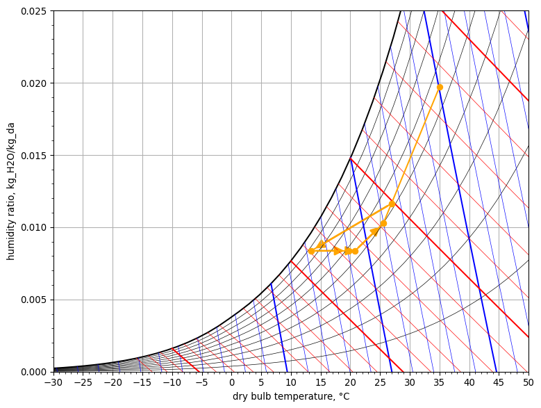
Psychrometric Chart#

psych_chart = PsychrometricChart(fig_size=(8, 6))

psych_chart.plot_process(
    name='adiabatic mixing',
    start_point=StatePoint(outdoor_air.Tdb, outdoor_air.W),
    end_point=StatePoint(zone_air.Tdb, zone_air.W),
    mix_point=StatePoint(mixed_air.Tdb, mixed_air.W)
)

psych_chart.plot_process(
    name='cooling coil',
    start_point=StatePoint(mixed_air.Tdb, mixed_air.W),
    end_point=StatePoint(cooled_air.Tdb, cooled_air.W)
)

# psych_chart.plot_process(
#     name='fan heating',
#     start_point=StatePoint(cooled_air.Tdb, cooled_air.W),
#     end_point=StatePoint(supply_air.Tdb, supply_air.W)
# )

psych_chart.plot_process(
    name='space',
    start_point=StatePoint(supply_air.Tdb, supply_air.W),
    end_point=StatePoint(zone_air.Tdb, zone_air.W)
)

psych_chart.show()

B. Summer Peak Design with High Latent Load#

We shall use the same design specifications as that of the CAV system analyzed under peak-load condition in Example 1 with one major difference. Instead of the space SHR being equal to 0.7, we are specified a value of 0.5, i.e., the sensible and latent loads are equal. The cooling coil leaving air temperature is as before, at 58F and 80% RH (the working conditions of the cooling coil, which are reflected by its ADP, remain unchanged). We will determine the supply air mass flow rate, and cooling coil and reheat coil loads in this case. The fan air temperature rise is ignored for simplicity. We will determine the supply air mass flow rate, and cooling coil and reheat coil loads in this case. The fan air temperature rise is ignored for simplicity.

0. Design Conditions#

The same design conditions as in section A apply, except the SHR of the zone.

SHR_zone = Q_(50, 'pct')

1. Determine the Supply Air Condition and Mass Flow Rate#

When we draw the space condition line on the psychrometric chart, we see that it does not intersect with the saturation line.

space_condition_line = SpaceConditionLine(
    space_air=zone_air,
    Q=Q_zone,
    SHR=SHR_zone
)

psych_chart = PsychrometricChart(fig_size=(8, 6))
psych_chart.plot_space_condition_line(
    start_point=space_condition_line.start_point(),
    end_point=space_condition_line.end_point(),
    space_point=space_condition_line.space_point()
)
psych_chart.plot_line(
    name='line1',
    start_point=StatePoint(Q_(-10, 'degC'), cooled_air.W.to('kg / kg')),
    end_point=StatePoint(Q_(40, 'degC'), cooled_air.W.to('kg / kg'))
)
psych_chart.plot_point(
    name='point1',
    point=StatePoint(cooled_air.Tdb.to('degC'), cooled_air.W.to('kg / kg'))
)
psych_chart.show()

If we decide to keep the state of the cooled air leaving the cooling coil the same as in section A, we can determine the required state of the supply air with the humidity ratio of the cooled air, knowing that this can’t change through the reheat coil and the supply fan:

zone = AirConditioningProcess(
    W_ai=cooled_air.W,
    air_out=zone_air,
    Q=Q_zone,
    SHR=SHR_zone
)
supply_air = zone.air_in
m_supply = zone.m_da

ja.display_list([
    f"supply air state: <b>{supply_air.Tdb.to('degF'):~P.1f} TDB, {supply_air.W.to('lb / lb'):~P.5f} lb<sub>w</sub>/lb<sub>da</sub></b>",
    f"supply air mass flow rate: <b>{m_supply.to('lb / hr'):~P.0f}</b>"
])

supply air state: 69.4 °F TDB, 0.00836 lb_w/lb_da
supply air mass flow rate: 28733 lb/h

From the figure above, we see that we will have to heat the cooled air leaving the cooling coil in order to arrive onto the space condition line.

2. Determine Fan Heat and Air State at Reheat Coil Exit#

supply_fan = Fan(
    air_out=supply_air,
    fan_pressure=Q_(3, 'inch_H2O_60F'),
    fan_efficiency=Q_(70, 'pct'),
    motor_efficiency=Q_(84, 'pct'),
    m_da=m_supply
)

reheat_air = supply_fan.air_in

ja.display_list([
    f"reheated air state: <b>{reheat_air.Tdb.to('degF'):~P.1f} TDB, {reheat_air.W.to('lb / lb'):~P.5f} lb<sub>w</sub>/lb<sub>da</sub></b>"
])

reheated air state: 67.5 °F TDB, 0.00836 lb_w/lb_da

3. Determine Reheat Coil Load#

reheat_coil = AirConditioningProcess(
    air_in=cooled_air,
    air_out=reheat_air,
    m_da=m_supply
)

ja.display_list([
    f"reheat coil load: <b>{reheat_coil.Q.to('Btu / hr'):~P.0f}</b>"
])

reheat coil load: 79716 Btu/h

4. Determine the Mixed Air Condition at the Entrance of the Cooling Coil#

m_recir = m_supply - m_vent

recir_air_str = AirStream(state=zone_air, m_da=m_recir)
mixed_air_str = AirStream(m_da=m_supply)

mixing_chamber = AdiabaticMixing(
    in1=outdoor_air_str,
    in2=recir_air_str,
    out=mixed_air_str
)
mixed_air = mixing_chamber.stream_out.state

ja.display_list([
    f"mixed air state: <b>{mixed_air.Tdb.to('degF'):~P.1f} TDB, {mixed_air.W.to('lb / lb'):~P.5f} lb<sub>w</sub>/lb<sub>da</sub></b>"
])

mixed air state: 80.5 °F TDB, 0.01163 lb_w/lb_da

5. Determine Cooling Coil Load#

cooling_coil = AirConditioningProcess(
    air_in=mixed_air,
    air_out=cooled_air,
    m_da=m_supply,
)

ja.display_list([
    f"cooling coil load: <b>{cooling_coil.Q.to('Btu / hr'):~P.0f}</b>"
])

cooling coil load: -273335 Btu/h

6. Check the Energy Balance of the Entire System#

Ventilation load

Q_vent = m_vent * (outdoor_air.h - zone_air.h)

ja.display_list([
    f"ventilation load: <b>{Q_vent.to('Btu / hr'):~P.0f}</b>"
])

ventilation load: 60577 Btu/h

Total heat input

Q_in_tot = Q_zone + Q_vent + supply_fan.Q + reheat_coil.Q

ja.display_list([
    f"total heat input: <b>{Q_in_tot.to('Btu / hr'):~P.0f}</b>"
])

total heat input: 273523 Btu/h

The total heat input must (approximately) be equal to the total heat extracted from the system in the cooling coil.

Psychrometric Chart#

psych_chart = PsychrometricChart(fig_size=(8, 6))

psych_chart.plot_process(
    name='adiabatic mixing',
    start_point=StatePoint(outdoor_air.Tdb, outdoor_air.W),
    end_point=StatePoint(zone_air.Tdb, zone_air.W),
    mix_point=StatePoint(mixed_air.Tdb, mixed_air.W)
)

psych_chart.plot_process(
    name='cooling coil',
    start_point=StatePoint(mixed_air.Tdb, mixed_air.W),
    end_point=StatePoint(cooled_air.Tdb, cooled_air.W)
)

psych_chart.plot_process(
    name='reheat coil',
    start_point=StatePoint(cooled_air.Tdb, cooled_air.W),
    end_point=StatePoint(reheat_air.Tdb, reheat_air.W)
)

psych_chart.plot_process(
    name='fan heating',
    start_point=StatePoint(reheat_air.Tdb, reheat_air.W),
    end_point=StatePoint(supply_air.Tdb, supply_air.W)
)

psych_chart.plot_process(
    name='space',
    start_point=StatePoint(supply_air.Tdb, supply_air.W),
    end_point=StatePoint(zone_air.Tdb, zone_air.W)
)

psych_chart.show()

C. Winter Peak Design#

Consider the CAV system analyzed under peak cooling load condition in Example 19.1. The same space is to be maintained at 72°F (25.5°C) and 50% RH. The total heating load of the space is 150,000 Btu/hr (44 kW) with an SHR of 0.8. The outdoor design condition is 40°F (4.4°C) dry bulb and 40% RH. The same amount of ventilation air (1000 ft³/min or 472 L/s) is needed. Design the necessary heating and humidification equipment assuming saturated steam at 200°F (93°C) is available and the supply airflow rate is kept at the summer design peak value of 17,140 lb/hr (2.2 kg/s). The supply air dry-bulb temperature should not exceed 105°F (40.5°C).

0. Design Conditions#

Zone air condition:

zone_air = HumidAir(Tdb=Q_(72.0, 'degF'), RH=Q_(50.0, 'pct'))

Heating load on winter peak design day:

Q_zone = Q_(-150_000, 'Btu / hr')  # minus sign: heat is removed from the room
SHR_zone = Q_(0.8, 'frac')

Outdoor air condition:

outdoor_air = HumidAir(Tdb=Q_(40, 'degF'), RH=Q_(40, 'pct'))

Ventilation air flow rate:

V_vent = Q_(1000, 'ft ** 3 / min')

Mass flow rate of supply air:

m_supply = Q_(17_140, 'lb / hr')

1. Determine the Condition of Mixed Air at Entrance of Preheat Coil#

Determine ventilation and recirculation mass flow rates

m_vent = outdoor_air.rho * V_vent
m_recir = m_supply - m_vent

ja.display_list([
    f"ventilation mass flow rate: <b>{m_vent.to('lb / hr'):~P.0f}</b>",
    f"recirculation mass flow rate: <b>{m_recir.to('lb / hr'):~P.0f}</b>",
])

ventilation mass flow rate: 4750 lb/h
recirculation mass flow rate: 12390 lb/h

Get mixed air condition from adiabatic mixing of outdoor ventilation air and recirculated air from space

outdoor_air_str = AirStream(state=outdoor_air, m_da=m_vent)
recir_air_str = AirStream(state=zone_air, m_da=m_recir)
mixed_air_str = AirStream(m_da=m_supply)

mixing_chamber = AdiabaticMixing(
    in1=outdoor_air_str,
    in2=recir_air_str,
    out=mixed_air_str
)
mixed_air = mixing_chamber.stream_out.state

ja.display_list([
    f"mixed air state: <b>{mixed_air.Tdb.to('degF'):~P.1f} TDB, {mixed_air.W.to('lb / lb'):~P.5f} lb<sub>w</sub>/lb<sub>da</sub></b>"
])

mixed air state: 63.1 °F TDB, 0.00663 lb_w/lb_da

2. Determine the Condition of Supply Air to the Zone#

zone = AirConditioningProcess(
    air_out=zone_air,
    m_da=m_supply,
    Q=Q_zone,
    SHR=SHR_zone
)
supply_air = zone.air_in

ja.display_list([
    f"supply air state: <b>{supply_air.Tdb.to('degF'):~P.1f} TDB, {supply_air.W.to('lb / lb'):~P.5f} lb<sub>w</sub>/lb<sub>da</sub></b>"
])

supply air state: 100.7 °F TDB, 0.00997 lb_w/lb_da

The humidity ratio of the supply air is greater than that of the mixed air. Consequently, we will need to humidify the mixed air to arrive at the required supply air state on the space condition line.

3. Determine the Amount of Steam in the Humidifier and the Condition of the Preheated Air#

Mass flow rate of steam
The needed mass flow rate of steam follows from the difference between the humidity ratio of the supply air and that of the mixed air.

m_steam = m_supply * (supply_air.W - mixed_air.W)

ja.display_list([
    f"steam injection rate: <b>{m_steam.to('lb / hr'):~P.3f}</b>"
])

steam injection rate: 57.230 lb/h

The steam injected in the air stream is saturated dry steam at a temperature of 200 °F.

Water = Fluid('Water')
steam = Water(T=Q_(200, 'degF'), x=Q_(100, 'pct'))

Humidification process
From the humidification process using steam injection the air state at the entrance of the humidifier can be determined. This is also the air state at the exit of the preheater. In a humidification process only water is added to the air stream; there is no heat transfer with the air stream, so Q needs to be set to zero in order to solve this air conditioning process.

humidifier = AirConditioningProcess(
    W_ai=mixed_air.W,
    air_out=supply_air,
    m_da=m_supply,
    h_w=steam.h,
    m_w=m_steam,
    Q=Q_(0, 'Btu / lb')
)
preheated_air = humidifier.air_in

ja.display_list([
    f"preheated air state: <b>{preheated_air.Tdb.to('degF'):~P.1f} TDB, {preheated_air.W.to('lb / lb'):~P.5f} lb<sub>w</sub>/lb<sub>da</sub></b>"
])

preheated air state: 100.1 °F TDB, 0.00663 lb_w/lb_da

4. Determine the Sensible Heating needed by the Preheat Coil#

The condition of the mixed air at the entrance of the preheat coil and the condition of the air at the exit of the preheat coil are known. The required heating capacity of the preheat coil on the winter peak design day can then be determined.

preheat_coil = AirConditioningProcess(
    air_in=mixed_air,
    air_out=preheated_air,
    m_da=m_supply
)

ja.display_list([
    f"preheat coil capacity: <b>{preheat_coil.Q.to('Btu / hr'):~P.0f}</b>"
])

preheat coil capacity: 154325 Btu/h

5. Check the Energy Balance of the Entire System#

Ventilation load

Q_vent = m_vent * (outdoor_air.h - zone_air.h)

ja.display_list([
    f"ventilation load: <b>{Q_vent.to('Btu / hr'):~P.0f}</b>"
])

ventilation load: -69347 Btu/h

Total energy output

Q_out_tot = Q_zone + Q_vent

ja.display_list([
    f"total heat loss: <b>{Q_out_tot.to('Btu / hr'):~P.0f}</b>"
])

total heat loss: -219347 Btu/h

Total heat input

Q_in_tot = preheat_coil.Q + m_steam * steam.h

ja.display_list([
    f"total heat input: <b>{Q_in_tot.to('Btu / hr'):~P.0f}</b>"
])

total heat input: 219895 Btu/h

Psychrometric Chart#

psych_chart = PsychrometricChart(fig_size=(8, 6))

psych_chart.plot_process(
    name='adiabatic mixing',
    start_point=StatePoint(outdoor_air.Tdb, outdoor_air.W),
    end_point=StatePoint(zone_air.Tdb, zone_air.W),
    mix_point=StatePoint(mixed_air.Tdb, mixed_air.W)
)

psych_chart.plot_process(
    name='preheat coil',
    start_point=StatePoint(mixed_air.Tdb, mixed_air.W),
    end_point=StatePoint(preheated_air.Tdb, preheated_air.W)
)

psych_chart.plot_process(
    name='steam injection',
    start_point=StatePoint(preheated_air.Tdb, preheated_air.W),
    end_point=StatePoint(supply_air.Tdb, supply_air.W)
)

psych_chart.plot_process(
    name='space',
    start_point=StatePoint(supply_air.Tdb, supply_air.W),
    end_point=StatePoint(zone_air.Tdb, zone_air.W)
)

psych_chart.show()

Air Conditioning Calculations with Python

Design of a Single-Zone CAV System

Contents

Design of a Single-Zone CAV System#

A. Summer Peak Design#

0. Design Conditions#

1. Determine the Supply Air Condition and Mass Flow Rate#

2. Determine the Mixed Air Condition at the Entrance of the Cooling Coil#

3. Determine Fan Heat and Air State at Cooling Coil Exit#

4. Determine Cooling Coil Load#

Psychrometric Chart#

B. Summer Peak Design with High Latent Load#

0. Design Conditions#

1. Determine the Supply Air Condition and Mass Flow Rate#

2. Determine Fan Heat and Air State at Reheat Coil Exit#

3. Determine Reheat Coil Load#

4. Determine the Mixed Air Condition at the Entrance of the Cooling Coil#

5. Determine Cooling Coil Load#

6. Check the Energy Balance of the Entire System#

Psychrometric Chart#

C. Winter Peak Design#

0. Design Conditions#

1. Determine the Condition of Mixed Air at Entrance of Preheat Coil#

2. Determine the Condition of Supply Air to the Zone#

3. Determine the Amount of Steam in the Humidifier and the Condition of the Preheated Air#

4. Determine the Sensible Heating needed by the Preheat Coil#

5. Check the Energy Balance of the Entire System#

Psychrometric Chart#